HSR Texas Geo Database Benchmark
The HSR Texas Spatial Database Benchmark - A Proposal
Date of first proposal: December 21, 2009. Status: Call for Comments and Call for Participation.
Inhaltsverzeichnis
Introduction
This is a proposal for a spatial database benchmark from the University of Applied Sciences Rapperswil (HSR). A study of existing database benchmarks revealed that there exists no information publicly available which compares spatial database systems regarding their performance. Spatial 'database management systems' (DMBS) typically form the persistence layer of a geographic information system (GIS).
Thus the Institute for Software at the University of Applied Sciences Rapperswil (HSR) decided to propose such a benchmark. This benchmark is being called 'The HSR Texas Spatial Database Benchmark' because it was defined from a HSR institute and because data comes from Texas USA.
The benchmark is based on a predefined set of queries. These queries consist of simple spatial queries, defined in the OpenGIS(tm) 'Simple Features Interface Standard (SFS)'. The queries are performed on different-sized data sets for monitoring the behavior on various loads as well as on different hardware systems.
In the following sections the methodology, the queries are explained and the used datasets are defined. This proposal concludes with a Call for Comments about the benchmark as well as a Call for Participation to apply and test this benchmark on existing DBMS software.
Methodology
The benchmark follows the below defined rules of engagement.
- Each test runs three times in a row, the results of the third run are used for the comparison: this benchmark assumes full system caches ('hot' benchmark).
- Each test takes place on the same machine.
- All other DBMS are shut down while the tests are running.
- Each DBMS has the same data which comes from real world data sets (as indicated below).
- The coordinate reference system used is spherical (geographical).
- Each test uses bounding box or point variables which are the same for the respective systems in the test. These variables are chosen at random from within the subset space.
Any hardware used needs to be specified according to following points:
- System Type
- Model
- Processor
- RAM
- Hard drive
- Operating system
There are two variants of the test: "No tuning/initial" and "Tuned".
- The variant "No tuning/initial" is mandatory in order to make benchmarks more widely applicable. The respective default installation of one DBMS is used.
- The variant "Tuned" is optional and needs proper documentation of all tuned parameters and activities.
Queries
The following queries are selected from the SQL functions defined by the SFS. The placeholder '{dataset}' will be substituted by the respective table names. The variable @bbox complies with randomly selected rectangular polygons in the geographical range of each data set, but which are the same for every system. The variable @point corresponds to a random point which is located in the area of the subsets. "geo" identifies the table column with geographical data. The following statements are given in pseudo SQL code.
Variable(s) @bbox:
- 'Aligned with grid': e.g.
POLYGON ((-101.3135 32.026, -101.3135 29.974, -98.7865 29.974, -98.7865 32.026, -101.3135 32.026)). - See chapter below.
Variable(s) @point:
- E.g.
POINT(-101.3135 32.026). - See chapter below.
Query 1. Loading the data
Create tiered data subsets by sub-dividing with a given bounding box '@bbox', creating the indices.
 SELECT * INTO {dataset}
 FROM {original dataset}
 WHERE ST_Intersects(@bbox, geo);
 CREATE SPATIAL INDEX idx ON {dataset} ([geo]);
Query 2. A Non-spatial Selection: Count
Count all railroads. We expect the 'roadflg' to have an index.
 SELECT count(*)
 FROM {dataset lines} l
 WHERE l.roadflg='Y';
Query 3. Spatial Selection I: Intersect Point, Line and Polygons
Count all a) points, b) lines, c) polygons that intersect with a given bounding box '@bbox'.
 a)
 SELECT count(*)
 FROM {dataset points} p
 WHERE ST_Intersects(@bbox, p.geo);
 b)
 SELECT count(*)
 FROM {dataset lines} l
 WHERE ST_Intersects(@bbox, l.geo);
 c)
 SELECT count(*)
 FROM {dataset polygons} pg
 WHERE ST_Intersects(@bbox, pg.geo);
Query 4. Spatial Selection II: Distance within
Count all a) points, b) lines, c) polygons that are within 20000 meters from a given point '@point'. Make sure the index is used, which usually needs a vendor specific implementation.
 a)
 SELECT count(*)
 FROM {dataset points} p
 WHERE ST_Distance(@point, geo) <= 20000;
 b)
 SELECT count(*)
 FROM {dataset lines} l
 WHERE ST_Distance(@point, geo) <= 20000;
 c)
 SELECT count(*)
 FROM {dataset polygons} pg
 WHERE ST_Distance(@point, geo) <= 20000;
Query 5. Spatial Selection III: Intersect/Join Lines and Polygons
Count all railroads that intersect with a water area. We expect the 'railflg' to have an index.
 SELECT count(*)
 FROM {dataset lines} l, areawater_full pg
 WHERE ST_Intersects(pg.geom, l.geom) = 1 AND l.railflg = 'Y';
Datasets
At the Free and Open Source Software for Geospatial Conference (FOSS4G) 2009, a 'Web Mapping Performance Shoot-out' was performed which compared the open source GIS software products GeoServer and MapServer ([1]). There, PostgreSQL/PostGIS and Oracle have been tested too. Several sets from the TIGER shapefiles of Texas that can be downloaded from the U.S. Census Bureau where used as data basis.
Download
- http://www.maptools.org/foss4g/ (user/pass: foss4g/foss4g)
- vector-data-tiger08-tx-merged.zip (1.1 GB) (TIGER 08, merged, for Texas)
- GNIS-2009.zip (7 MB) (2009 GNIS point data for Texas)
This data is proposed to use within this benchmark containing rivers, roads, railroads, Points-of-interest and water areas. The data originate from the following shape files:
| Shape file name | gnis_names09 | edges_merge | areawater_merge |
|---|---|---|---|
| Type | Point | Multilinestring | Multipolygon |
| Number of records | 103,000 | Over 5 M | 380,000 |
| SRID | EPSG:4326 | EPSG:4326 | EPSG:4326 |
| Source | GNIS database | TIGER 2008 | TIGER 2008 |
| Description | All locations and Point of interest for the state of Texas. | All line elements (rivers and roads) from the TIGER 2008 dataset for the state of Texas. | The TIGER set of polygons describing water surface for the state of Texas. |
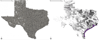
These data sets are divided by a bounding-box procedure to subsets. Using these subsets the behavior of the respective DBMS can be observed in different-sized data sets. The figure to the right shows the gnis_names09 data set (left) and the areawater_merge data set (right).
It follows the definition of the (sub-)datasets (coordinates in WGS94):
Point data gnis_names09
| Subset | Number of records | Bounding box |
|---|---|---|
| gnis_names_40000 | 40,002 | ST_MakeBox2D(ST_MakePoint(-103.208, 28.435), ST_MakePoint(-96.891, 33.460)) |
| gnis_names_60000 | 60,001 | ST_MakeBox2D(ST_MakePoint(-104.006, 27.787), ST_MakePoint(-96.093, 34.193)) |
| gnis_names_80000 | 80,001 | ST_MakeBox2D(ST_MakePoint(-104.904, 27.058), ST_MakePoint(-95.195, 34.830)) |
| gnis_names_100000 | 100,002 | ST_MakeBox2D(ST_MakePoint(-106.168, 26.032), ST_MakePoint(-93.932, 35.693)) |
Multilinestring data edges_merge
| Subset | Number of records | Bounding box |
|---|---|---|
| edges_500000 | 500,161 | ST_MakeBox2D(ST_MakePoint(-102.169, 29.279), ST_MakePoint(-97.930, 30.515)) |
| edges_1000000 | 1,000,200 | ST_MakeBox2D(ST_MakePoint(-103.109, 28.516), ST_MakePoint(-96.991, 30.580)) |
| edges_1500000 | 1,500,680 | ST_MakeBox2D(ST_MakePoint(-103.518, 28.183), ST_MakePoint(-96.581, 31.255)) |
| edges_2000000 | 2,000,250 | ST_MakeBox2D(ST_MakePoint(-104.605, 27.301), ST_MakePoint(-95.494, 30.945)) |
| edges_2500000 | 2,500,450 | ST_MakeBox2D(ST_MakePoint(-106.041, 26.134), ST_MakePoint(-94.058, 30.754)) |
Multipolygon data areawater_merge
| Subset | Number of records | Bounding box |
|---|---|---|
| areawater_100000 | 100,025 | ST_MakeBox2D(ST_MakePoint(-102.789, 28.775), ST_MakePoint(-97.3102, 33.174)) |
| areawater_150000 | 150,038 | ST_MakeBox2D(ST_MakePoint(-103.261, 28.391), ST_MakePoint(-96.8380, 33.556)) |
| areawater_200000 | 200,019 | ST_MakeBox2D(ST_MakePoint(-103.674, 28.057), ST_MakePoint(-96.4257, 33.814)) |
| areawater_250000 | 250,005 | ST_MakeBox2D(ST_MakePoint(-104.272, 27.571), ST_MakePoint(-95.8272, 34.041)) |
| areawater_300000 | 300,014 | ST_MakeBox2D(ST_MakePoint(-104.691, 27.230), ST_MakePoint(-95.4083, 34.451)) |
| areawater_350000 | 350,002 | ST_MakeBox2D(ST_MakePoint(-105.536, 26.545), ST_MakePoint(-94.5637, 35.042)) |
Runtime variables for Queries 3 and 4
Bounding Box data for Query 3 (correspond to an area of about 50% of the elements from the respective subarea)
- Points:
 Points 40000:   ST_MakeBox2D(ST_MakePoint(-102.311, 29.164), ST_MakePoint(-97.789, 32.836))
 Points 60000:   ST_MakeBox2D(ST_MakePoint(-102.7765, 28.786), ST_MakePoint(-97.3235, 33.214))
 Points 80000:   ST_MakeBox2D(ST_MakePoint(-103.1755, 28.462), ST_MakePoint(-96.9245, 33.538))
 Points 100000:  ST_MakeBox2D(ST_MakePoint(-103.508, 28.192), ST_MakePoint(-96.592, 33.808))
- Lines:
 Line 500000:    ST_MakeBox2D(ST_MakePoint(-101.743755, 29.62462), ST_MakePoint(-98.356245, 32.37538))
 Line 1000000:   ST_MakeBox2D(ST_MakePoint(-102.0982, 29.3368), ST_MakePoint(-98.0018, 32.6632))
 Line 1500000:   ST_MakeBox2D(ST_MakePoint(-102.54375, 28.975), ST_MakePoint(-97.55625, 33.025))
 Line 2000000:   ST_MakeBox2D(ST_MakePoint(-102.9893, 28.6132), ST_MakePoint(-97.1107, 33.3868))
 Line 2500000:   ST_MakeBox2D(ST_MakePoint(-103.242, 28.408), ST_MakePoint(-96.858, 33.592))
- Polygons:
 Polygon 100000: ST_MakeBox2D(ST_MakePoint(-102.227875, 29.2315), ST_MakePoint(-97.872125, 32.7685))
 Polygon 150000: ST_MakeBox2D(ST_MakePoint(-102.54375, 28.975), ST_MakePoint(-97.55625, 33.025))
 Polygon 200000: ST_MakeBox2D(ST_MakePoint(-102.79645, 28.7698), ST_MakePoint(-97.30355, 33.2302))
 Polygon 250000: ST_MakeBox2D(ST_MakePoint(-103.00925, 28.597), ST_MakePoint(-97.09075, 33.403))
 Polygon 300000: ST_MakeBox2D(ST_MakePoint(-103.2686, 28.3864), ST_MakePoint(-96.8314, 33.6136))
 Polygon 350000: ST_MakeBox2D(ST_MakePoint(-103.47475, 28.219), ST_MakePoint(-96.62525, 33.781))
Point data for Query 4
- Points:
 Points 40000:   ST_MakePoint(-102.311, 32.836)
 Points 60000:   ST_MakePoint(-102.7765, 33.214)
 Points 80000:   ST_MakePoint(-103.1755, 33.538)
 Points 100000:  ST_MakePoint(-103.508, 33.808)
- Lines:
 Line 500000:    ST_MakePoint(-101.743755, 30.37538)
 Line 1000000:   ST_MakePoint(-102.0982, 30.4632)
 Line 1500000:   ST_MakePoint(-102.54375, 31.025)
 Line 2000000:   ST_MakePoint(-102.9893, 29.3868)
 Line 2500000:   ST_MakePoint(-103.242, 30.592)
- Polygons:
 Polygon 100000: ST_MakePoint(-101.227, 30.7685)
 Polygon 150000: ST_MakePoint(-102.54375, 32.025)
 Polygon 200000: ST_MakePoint(-102.79645, 32.2302)
 Polygon 250000: ST_MakePoint(-102.009, 32.951)
 Polygon 300000: ST_MakePoint(-102.2686, 32.1136)
 Polygon 350000: ST_MakePoint(-102.47475, 33.781)
Scripts for benchmark automation
tbd.
Call for Comments and Call for Participation
The 'HSR Texas Spatial Database Benchmark' was conducted and verified by a first time in December 2009 during a Master Seminar by the Institute for Software at HSR. Two database management systems software (DBMS), one commercially available (Microsoft SQL Server 2008 Spatial) an one under an Open Source license (PostgreSQL 8.4.1/PostGIS 1.4.0), have been chosen. The results are currently evaluated and will probably be published in 2010.
Two actions from researchers and volunteers may complement this research:
- Submit comments on the 'HSR Texas Spatial Database Benchmark' itself.
- Do further experiments on existing DBMS.
We are looking forward for a fruitful discussion!
Feedback, Discussion and Contact
Please direct any comments either to the discussion page, to the OSGEOs benchmarking mailing list - or directly to Prof. S. Keller from Institute for Software at HSR.
Weblinks
- GeoServer vs. MapServer Benchmark 2009
- List of benchmarks and performance tests: http://delicious.com/sfkeller/database+benchmark
- http://trac.osgeo.org/postgis/wiki/DevWikiGardenTest

